Outputs and Visualization

After the execution of the SURFATT_tomo, the outputs of the tomography are stored in the directory that is specified in the input parameter file. The outputs include the following files:

Output files

final_model.h5

The final model file. It always contains the grid axes:

• x: Longitude of the model in degree with the shape of (nx)
• y: Latitude of the model in degree with the shape of (ny)
• z: Depth of the model in km with the shape of (nz)

together with the model fields, each with the shape of (nx, ny, nz). Which fields are present depends on inversion.model_para_type:

In all three cases vp and rho are added when inversion.use_alpha_beta_rho is True.

initial_model.h5, written when output_initial_model is True.

objective_function.txt

One header line followed by one line per iteration, with 11 whitespace-separated columns:

The residual columns of data types that are not activated are filled with zeros.

model_iter.h5 — model and gradient history

model_iter.h5 is written when output_in_process_model is True, or whenever optim_method is 1 (L-BFGS), which needs the history to build its search direction.

Besides the same x, y and z axes as final_model.h5, it holds, for every iteration {NNN} (three digits, zero-padded):

• model_vs_{NNN}: S-wave velocity model of iteration {NNN} in km/s, with the shape of (nx, ny, nz)
• grad_vs_{NNN}: Preconditioned gradient of iteration {NNN}, with the shape of (nx, ny, nz)

model_vp and model_rho (use_alpha_beta_rho: True), model_gc and model_gs (model_para_type: 1), and model_gamma (model_para_type: 2) are stored alongside.

src_rec_file_forward_*.csv — forward travel times

src_rec_file_forward_{RL|LV}_{PH|GR}_{NNN}.csv holds the synthetic travel-time data of iteration {NNN}, with one file per activated wave type (RL Rayleigh, LV Love) and velocity type (PH phase, GR group). In forward-only mode (SURFATT_tomo -f) the iteration suffix is omitted.

Visualization

we recommend using the PyGMT package to visualize the outputs of the tomography. Please refer to examples/xxxx/plot_model.ipynb for examples to visualize the final model.

Rotate the model back to the original coordinate system

If the topography, the sources, and the receivers are rotated before the inversion, you can use the SURFATT_rotate_model command to rotate the model back to the original coordinate system. The command is called as follows:

Usage: SURFATT_rotate_model -i model_file -o out_file -c clat/clon [-a angle] [-k keyname] [-h]

 Rotate a model from the local (rotated) frame back to geographic
 coordinates and convert to csv format.

 required arguments:
  -i model_file        Path to model file in HDF5 format
  -o out_file          Output csv file name
  -c clat/clon         Centre of rotation (lat/lon)

 optional arguments:
  -a angle             Rotation angle in degrees (default: 0)
  -k keyname           Export only this scalar dataset as the model column
                       One of: vs, vsv, vsh, vp, rho, zeta, gamma
                       optionally with a model_/grad_ prefix and an _NNN
                       iteration suffix, e.g. model_vs_042 in model_iter.h5
                       The csv column is named after the bare field, so
                       model_vs_042 is written as a column named vs
                       Without -k, vs is exported together with whichever
                       anisotropy fields the file carries: g0/theta for
                       azimuthal, vsv/zeta for radial
  -h                   Print help message

For the Hawaii example, we can rotate the final model back to the original coordinate system using the following command:

angle_back=30
pos_str=19.5/-155.5
 
SURFATT_rotate_model -i OUTPUT_FILES/final_model.h5 -a $angle_back -c $pos_str -o OUTPUT_FILES/final_model.csv

The rotated model is stored in the final_model.csv file with 4 columns: lon, lat, depth, and vs. When -k is omitted and the model carries anisotropy, the columns g0 and theta (azimuthal) or vsv and zeta (radial) are appended.

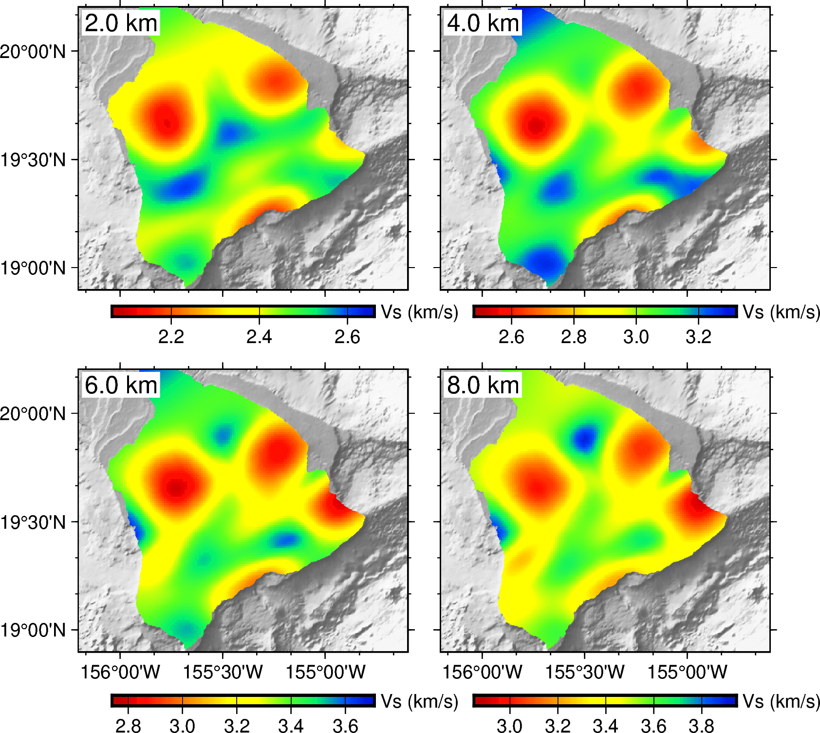
The following is an example script to visualize the final model by reading this final_model.csv:

import pygmt
import numpy as np
import pandas as pd
 
# Load the final model
fm_tab = pd.read_csv("./OUTPUT_FILES/final_model.csv")
z = np.unique(fm_tab["depth"].values)
 
# Plot the final model
fig = pygmt.Figure()
region=[-156.2, -154.6, 18.9, 20.2]
dep = [2, 4, 6, 8]
pygmt.config(MAP_FRAME_TYPE="plain")
with fig.subplot(nrows=2, ncols=2, figsize=("12c", "12c"), sharex='b', sharey='l', frame=["af", "WSne"]):
    for i, depth in enumerate(dep):
        close_dep = z[np.abs(z-depth).argmin()]
        data = fm_tab[fm_tab["depth"]==close_dep]
        fig.basemap(region=region, projection="M?", panel=i)
        grid = pygmt.grdcut("@earth_relief_15s", region=region)
        pygmt.makecpt(cmap="gray", series=[-6000, 9000, 10], reverse=True)
        fig.grdimage(grid, region=region, projection="M?", cmap=True, shading=True)
        grid = pygmt.surface(x=data['lon'], y=data['lat'], z=data['vs'], region=region, spacing="0.01" )
        vmax = data['vs'].max()+0.05; vmin = data['vs'].min()-0.05
        pygmt.makecpt(cmap="seis", series=[vmin, vmax])
        fig.coast(area_thresh=10, resolution='f', land=True)
        fig.grdimage(grid=grid, cmap=True)
        fig.coast(Q=True)
        fig.text(text=f'{close_dep} km', position='TL', justify='TL', offset='0.1c/-0.1c', fill='white', font='12p')
        fig.colorbar(frame=['a0.2g0.2', 'y+l"Vs (km/s)"'])
fig.show()