Travel-time data preparation

Tabular travel-time data format

The travel-time data can be obtained from the observed surface wave dispersion. The travel-time data should be stored in a csv file with the following columns:

• tt: travel time from the source to the receiver
• staname: station name
• stla: latitude of the station
• stlo: longitude of the station
• evtname: event name
• evla: latitude of the event
• evlo: longitude of the event
• period: period of the surface wave
• weight: weight of the travel-time data
• dist: distance between the source and receiver (optional)
• vel: phase or group velocity of the surface wave (optional)

A template of the travel-time data file can be found here.

Rotate receiver locations by a given angle

Why rotate?

The computational domain of SurfATT is a rectangle aligned with the longitude and latitude axes — either given explicitly through domain.grid_method_1 (lon_min_max / lat_min_max), or derived from the bounding box of all sources and receivers padded by num_grid_margin cells (grid_method_0).

Many study regions are elongated along an oblique direction. Rotating the sources and receivers so that the long axis of the array lines up with one of the coordinate axes lets a much tighter rectangle enclose the same data:

Two further points make this safe and useful:

• SURFATT_rotate_src_rec applies a rigid rotation of the sphere (the reference point clat/clon is moved to (0°, 0°), then the array is spun about it by angle). Great-circle distances between any pair of points — and hence the observed travel times — are unchanged, so the inverse problem is identical, only more efficiently gridded.
• Because the rotated frame is centred on the equator, cos(latitude) ≈ 1 over the whole domain, so a grid interval of d degrees in longitude and latitude gives nearly square cells in km. In the original frame at mid-to-high latitudes the same interval produces cells that are noticeably narrower in the longitude direction.

Command SURFATT_rotate_src_rec

The SURFATT_rotate_src_rec command is used to rotate the location of sources and receivers by a given angle. The command is called as follows:

 Usage: SURFATT_rotate_src_rec -i src_rec_file -a angle -c clat/clon [-h] [-o out_file]

 Rotate source and receiver locations by a given angle (anti-clockwise)

 required arguments:
  -i src_rec_file      Path to src_rec file in csv format
  -a angle             Rotation angle in degrees
  -c clat/clon         Centre of rotation (lat/lon)

 optional arguments:
  -h                   Print help message
  -o out_file          Output file name (default: input file + "_rot")

The SURFATT_rotate_src_rec command reads the source and receiver locations from the input file src_rec_file and rotates them by the given angle angle (in anti-clockwise degrees) about the center of rotation clat/clon. The rotated source and receiver locations are written to the output file out_src_rec_file. If the output file is not specified, the rotated source and receiver locations are written to a file with the name src_rec_file appended with _rot.

Example

In the following example, the source and receiver locations are rotated by -30 degrees about the center of rotation (19.5, -155.5) and written to the output file src_rec_file_rotated.csv. To illustrate this example, we use Jupyter Notebook to invoke the SURFATT_rotate_src_rec command, and plot the original and rotated source and receiver locations.

First, we import the required Python packages:

import pandas as pd
import matplotlib.pyplot as plt
import cartopy.crs as ccrs
import cartopy.feature as cfeature

A function to plot the source and receiver locations is defined as follows:

def plot_basemap(region, feature=True):
    fig = plt.figure()
    ax = fig.add_subplot(1, 1, 1, projection=ccrs.Mercator())
    ax.set_extent(region, crs=ccrs.PlateCarree())
    gl = ax.gridlines(crs=ccrs.PlateCarree(), draw_labels=True,
                      linewidth=1, color='gray', alpha=0.5, linestyle='--')
    if feature:
        ax.coastlines()
        # plot land
        ax.add_feature(cfeature.LAND)
    return ax

Next, we read the source and receiver locations from the input file src_rec_file.csv and plot them:

sr = pd.read_csv('src_rec_file.csv')
ax = plot_basemap([-156.3, -154.7, 18.8, 20.4])
ax.plot(sr['stlo'], sr['stla'], 'r^', markersize=5, transform=ccrs.PlateCarree())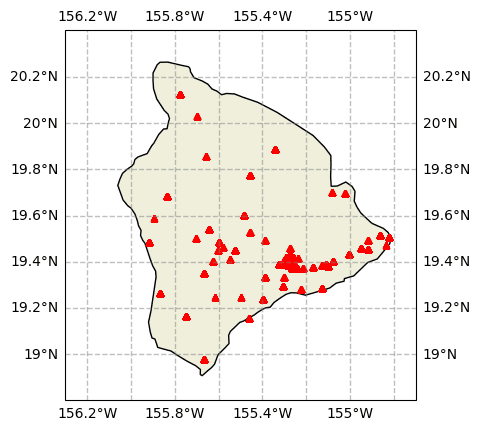

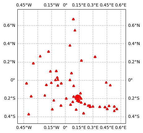
The source and receiver locations are then rotated by -30 degrees about the center of rotation (19.5, -155.5) and written to the output file src_rec_file_rotated.csv:

! SURFATT_rotate_src_rec -i src_rec_file.csv -a -30 -c 19.5/-155.5 -o src_rec_file_rotated.csv

Finally, we read the rotated source and receiver locations from the output file src_rec_file_rotated.csv and plot them:

sr_rotated = pd.read_csv('src_rec_file_rotated.csv')
minx = sr_rotated['stlo'].min()
maxx = sr_rotated['stlo'].max()
miny = sr_rotated['stla'].min()
maxy = sr_rotated['stla'].max()
marginx = (maxx - minx) * 0.1
marginy = (maxy - miny) * 0.1
region = [minx - marginx, maxx + marginx, miny - marginy, maxy + marginy]
ax = plot_basemap(region, feature=False)
ax.plot(sr_rotated['stlo'], sr_rotated['stla'], 'r^', markersize=5, transform=ccrs.PlateCarree())